A Simple Simulation • ZINB.GP

Using ZINB.GP’s ZINB_GP model

First, we import our package as well as some dependencies we will use to simulate the dataset.

library(mvtnorm)
library(Matrix)
library(ZINB.GP)

Generating a dataset

We go through the full process to generate the dataset in an attempt to provide clarity on what the various matrix parameters passed into ZINB_GP are.

Helper functions

First we will define a few helper functions. The first will create Vs and Vt, the spatial and temporal design matrices. These will consit of indicator variables indicating at which point in space/time our data points are.

make_Vs_Vt <- function(num_spatial, num_temporal, avg_obs) {
    n_time_points <- num_temporal # Number of temporal units
    n_unit_mat <- matrix(rpois(num_spatial * n_time_points, avg_obs), nrow = num_spatial, byrow = TRUE) # sample around avg_obs observations per sampling unit (both space and time)

    N <- sum(n_unit_mat)    # Total number of observations
    id <- c()
    for (i in seq_len(nrow(n_unit_mat))) {
        id <- c(id, rep(i, sum(n_unit_mat[i, ])))
    }

    tp_seq <- c()
    for (j in seq_len(ncol(n_unit_mat))) {
        tp_seq <- c(tp_seq, rep(j, sum(n_unit_mat[, j])))
    }

    # spatial design matrix
    Vs <- as.matrix(sparseMatrix(i = 1:N, j = id, x = rep(1, N)))

    # temporal design matrix
    Vt <- as.matrix(sparseMatrix(i = 1:N, j = tp_seq, x = rep(1, N)))

    return(list(Vs = Vs, Vt = Vt, N = N))
}

Next, we will make some functions to generate the spatial and temporal random effects (varying intercepts) and the corresponding distance matrices.

make_spatial_effects <- function(phi_nb, phi_bin, sigma_bin_s, sigma_nb_s, coords) {
    ##########################
    # Spatial Random Effects #
    ##########################
    Ds <- as.matrix(dist(coords))
    Ks_bin <- sigma_bin_s^2 * exp(-phi_bin * Ds)
    Ks_nb <- sigma_nb_s^2 * exp(-phi_nb * Ds)
    a <- t(rmvnorm(n = 1, sigma = Ks_bin))
    c <- t(rmvnorm(n = 1, sigma = Ks_nb))

    return(list(a = a, c = c, Ds = Ds))
}

make_temporal_effects <- function(l1t, l2t, sigma1t, sigma2t, n_time_points) {
    ###########################
    # Temporal Random Effects #
    ###########################
    w <- matrix(1:n_time_points, ncol = 1)
    Dt <- as.matrix(dist(w))
    
    Kt_bin <- sigma1t^2 * exp(-Dt / (l1t^2))
    Kt_nb <- sigma2t^2 * exp(-Dt / (l2t^2))
    
    b <- t(rmvnorm(n = 1, sigma = Kt_bin))
    d <- t(rmvnorm(n = 1, sigma = Kt_nb))
    
    return(list(b = b, d = d, Dt = Dt))
}

Actually Generating the Data

Now we are ready to generate the dataset. First we define the number of spatial and temporal points we will be using.

num_spatial <- 30
num_temporal <- 10

Then, we create the spatial and temporal design matrices.

# Get Spatial and temporal design matrices, and total number of observations
out <- make_Vs_Vt(num_spatial, num_temporal, 2)
Vs <- out$Vs
Vt <- out$Vt
N  <- out$N     # Total number of observations

Then, we will generate the spatial coordinates, and the main predictors of interest X.

coords <- cbind(runif(num_spatial), runif(num_spatial))
x <- rnorm(N, 0, 1)
X <- as.matrix(x) # Design matrix, can add additional covariates (e.g., race, age, gender)
X <- cbind(1, X)
p <- ncol(X)

Next, we create the spatial and temporal distance matrices, and the spatial and temporal random effects.

phi_nb <- 1
phi_bin <- 2        # Spatial Kernel length scale for Gaussian processes in the logistic regression and negative binomial parts of the model
sigma_bin_s <- 1    
sigma_nb_s <- 1     # Overall spatial kernel Scale for GPs
out <- make_spatial_effects(phi_nb, phi_bin, sigma_bin_s, sigma_nb_s, coords)
a <- out$a
c <- out$c          # Spatial random effects
Ds <- out$Ds        # Spatial Distance matrix

l1t <- 2
l2t <- 3            # Temporal Kernel length scale
sigma1t <- 0.5
sigma2t <- 0.5      # Overall temporal kernel scale for GPs
out <- make_temporal_effects(l1t, l2t, sigma1t, sigma2t, num_temporal)
b <- out$b
d <- out$d          # Temporal random effects
Dt <- out$Dt        # Temporal distance matrix

Then we define the fixed effects (coefficients on X) for the logistic regression and the negative binomial models.

# LR Part
alpha <- c(-0.25, 0.25)

# NB Part
beta <- c(.5, -.25)

Then, we generate some spatial and temporal noise terms that will be added into the mix

sigma_eps1s <- sigma_eps2s <- 0.05
eps1s <- t(rmvnorm(n = 1, sigma = diag(sigma_eps1s^2, nrow = num_spatial)))
eps2s <- t(rmvnorm(n = 1, sigma = diag(sigma_eps2s^2, nrow = num_spatial)))

sigma_eps1t <- sigma_eps2t <- 0.05
eps1t <- t(rmvnorm(n = 1, sigma = diag(sigma_eps1t^2, nrow = num_temporal)))
eps2t <- t(rmvnorm(n = 1, sigma = diag(sigma_eps2t^2, nrow = num_temporal)))

Finally, we can create our models. First we simulate whether or not you are in the at risk group with a traditional logistic regression setting:

phi1 <- Vs %*% a + Vt %*% b
eta1 <- X %*% alpha + phi1 + Vs %*% eps1s + Vt %*% eps1t

p_at_risk <- exp(eta1) / (1 + exp(eta1)) # 1-pr("structural zero")
u <- rbinom(N, 1, p_at_risk[, 1]) # at-risk indicator

Then, if you are in the at-risk group, we draw the value at that point from a negative binomial distribution, in a GLM setting with logit link.

phi3 <- Vs %*% c + Vt %*% d
eta2 <- X[u == 1, ] %*% beta + phi3[u == 1, ] + Vs[u == 1, ] %*% eps2s + Vt[u == 1, ] %*% eps2t # Linear predictor for count part
N1 <- sum(u == 1)

r <- 1 # NB dispersion
psi <- exp(eta2) / (1 + exp(eta2)) # Prob of success

mu <- r * psi / (1 - psi) # NB mean
y <- rep(0, N) # Response
y[u == 1] <- rnbinom(N1, r, mu = mu[, 1]) # If at risk, draw from NB

Running the model on the generated dataset

Now we are ready to run the model. This is done as follows:

# Run for a short time for demo purposes
output <- ZINB_GP(X, y, coords, Vs, Vt, Ds, Dt, M = 10, 200, 100, 1, TRUE)
predictions <- output$Y_pred
sim_alpha <- output$Alpha
sim_beta <- output$Beta

Then we can investigate the output as desired, as an example, we create 90% CIs for alpha and beta, and investigate how often some samples were selected to be at risk.

Looking at 90% CIs for coefficients for the at-risk LR model:

alpha
#> [1] -0.25  0.25
aCIs <- apply(sim_alpha, 2, function(x) quantile(x, probs=c(0.05, 0.95)))
boxplot(aCIs, main = "CIs for Alpha")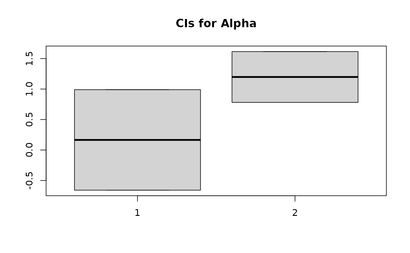

Looking at 90% CIs for coefficients for the NB model:

beta
#> [1]  0.50 -0.25
bCIs <- apply(sim_beta, 2, function(x) quantile(x, probs=c(0.05, 0.95)))
boxplot(bCIs, main = "CIs for Beta")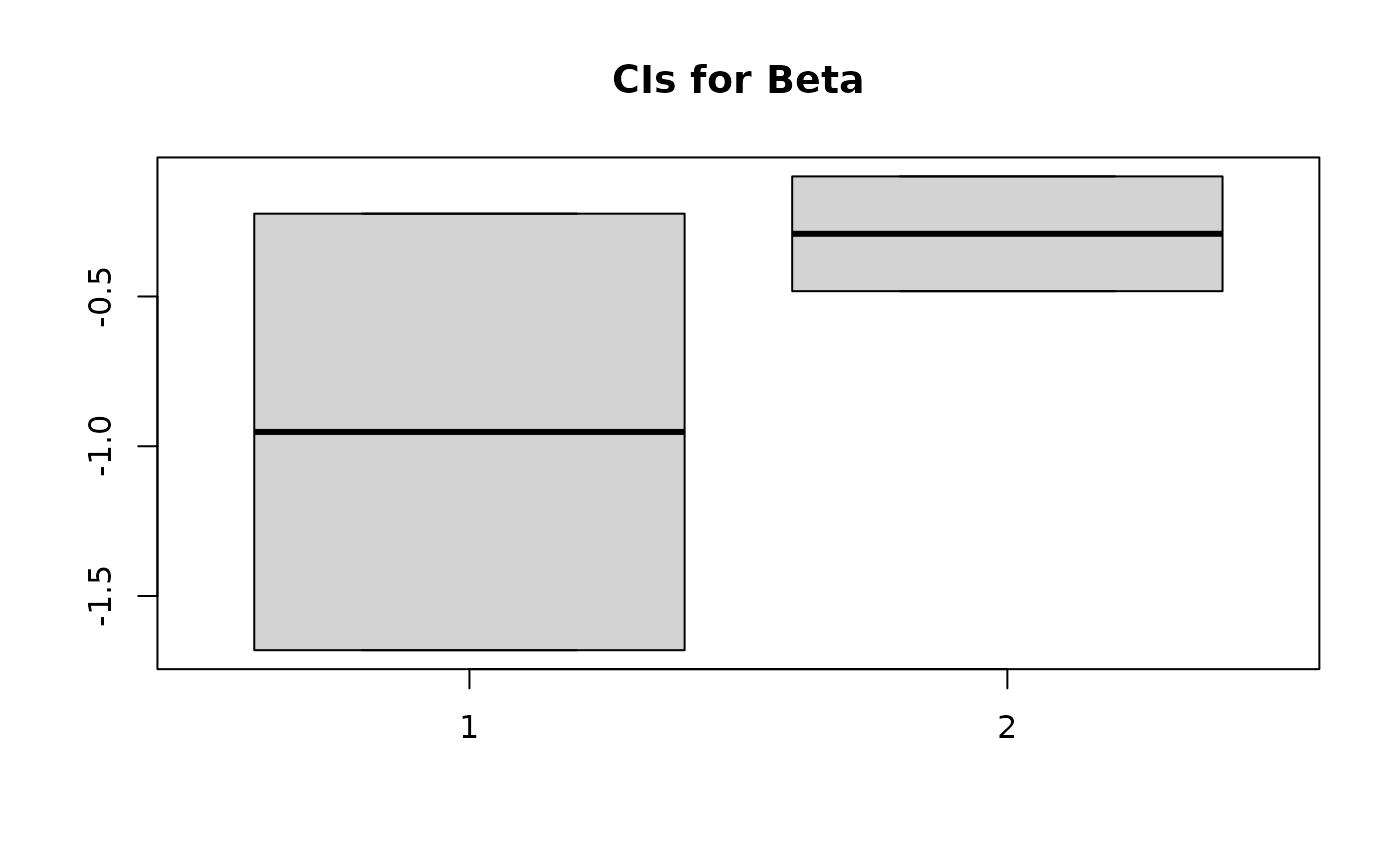

Viewing the frequency a few samples were at risk:

# Examine how often various samples are at risk
at_risk <- output$at_risk
sim_p_at_risk <- apply(at_risk, 2, mean)
sim_p_at_risk[1:20]
#>  [1] 0.25 0.15 0.07 1.00 0.71 0.87 1.00 0.94 0.68 0.83 0.69 0.35 0.16 1.00 0.82
#> [16] 0.44 0.60 1.00 0.94 1.00