Demonstration of ZINB_GP with Simulated Spatial-Temporal Data

Overview

This document demonstrates the use of the ZINB_GP function from the ZINB.GP package, which implements a Zero-Inflated Negative Binomial (ZINB) model with Gaussian Processes (GP) for spatial-temporal data. The package is sourced from GitHub: KingJMS1/NNGP_ZINB_R. We will simulate spatial and temporal data, then apply the ZINB_GP function to model it.

Loading Required Libraries

Load the necessary libraries for this demonstration.

library(ZINB.GP)
library(mvtnorm)
library(Matrix)
set.seed(123)    # For reproducibility

Simulating Spatial-Temporal Data

We will simulate data with spatial and temporal components. Assume we have:

n_locs: Number of spatial locations n_times: Number of time points X: Covariate matrix y: Response variable (counts with excess zeros) coords: Spatial coordinates Vs, Vt: Spatial and temporal variance components Ds, Dt: Spatial and temporal distance matrices Step 1: Define Parameters t

n_locs <- 10    # Number of spatial locations
n_times <- 10   # Number of time points
n <- n_locs * n_times  # Total number of observations
M <- 3          # Number of nearest neighbors for NNGP
nsim <- 400    # Number of MCMC simulations
burn <- 200     # Burn-in period

Step 2: Simulate Spatial Coordinates

Generate random spatial coordinates in a 10x10 grid.

coords <- cbind(runif(n_locs, 0, 10), runif(n_locs, 0, 10))
plot(coords, pch = 19, xlab = "X", ylab = "Y", main = "Simulated Spatial Locations")

Step 3: Simulate Covariates

Create a simple covariate matrix X with an intercept and one predictor.

X <- matrix(c(rep(1, n), rnorm(n)), ncol = 2)
colnames(X) <- c("Intercept", "X1")
head(X)
#>      Intercept         X1
#> [1,]         1  1.2240818
#> [2,]         1  0.3598138
#> [3,]         1  0.4007715
#> [4,]         1  0.1106827
#> [5,]         1 -0.5558411
#> [6,]         1  1.7869131

Step 4: Simulate Spatial and Temporal Effects

Simulate spatial and temporal covariance matrices using an exponential decay function.

# Number of locations and time points
n_locs <- 10    # spatial locations
n_times <- 10   # time points
n <- n_locs * n_times  # total observations

# Generate spatial coordinates for 10 locations
coords <- cbind(runif(n_locs, 0, 10), runif(n_locs, 0, 10))

# Create a time vector (assuming evenly spaced time points)
time_points <- seq(1, n_times)

# Expand spatial coordinates: repeat each spatial location for each time point
# Not actually necessary for use of package, just for later analysis
coords_st <- do.call(rbind, replicate(n_times, coords, simplify = FALSE))
# Create a time index for each observation
time_index <- rep(time_points, each = n_locs)

# Recompute the full spatial distance matrix for all observations (100 x 100)
Ds <- as.matrix(dist(coords))

# Compute the full temporal distance matrix for all observations (100 x 100)
Dt <- as.matrix(dist(time_points))

# Create spatial and temporal design matrices, indicates which observations
# correspond to which positions spatially and temporally
Vs <- as.matrix(sparseMatrix(i = 1:n, j = rep(1:10, 10), x = rep(1, n)))
Vt <- as.matrix(sparseMatrix(i = 1:n, j = time_index, x = rep(1, n)))

# Create spatial and temporal covariance matrices
# Initialize kernel parameters
cov_scale <- 0.5
dist_scale_space <- 0.3
dist_scale_time <- 2
# Spatial 
Cs <- (cov_scale^2) * exp(-dist_scale_space * Ds)
# Temporal
Ct <- (cov_scale^2) * exp(-Dt / (dist_scale_time ^ 2))

Step 5: Simulate Response Variable

Generate a ZINB response variable with spatial-temporal effects.

# Simulate latent spatial-temporal effects
err <- 0.1
spatial_effect <- rmvnorm(n = 1, sigma = Cs + diag(err, 10))
temporal_effect <- rmvnorm(n = 1, sigma = Ct + diag(err, 10))
eta <- X %*% c(1, 0.5) + Vs %*% t(as.matrix(spatial_effect)) + Vt %*% t(as.matrix(temporal_effect))

# ZINB parameters
phi <- 2  # Dispersion parameter
pi <- plogis(-1 + 0.3 * X[, 2])  # Zero-inflation probability
mu <- exp(eta)  # Mean of NB component

# Simulate ZINB data
y <- numeric(n)
for (i in 1:n) {
  if (runif(1) < pi[i]) {
    y[i] <- 0  # Zero-inflated part
  } else {
    y[i] <- rnbinom(1, size = phi, mu = mu[i])  # NB part
  }
}

# Expand coords for spatial-temporal grid
coords_st <- expand.grid(x = coords[, 1], y = coords[, 2], t = time_points)
coords_st <- as.matrix(coords_st[, 1:2])  # Only spatial coords for NNGP

# Summary of y
summary(y)
#>    Min. 1st Qu.  Median    Mean 3rd Qu.    Max. 
#>    0.00    0.00    1.00    2.59    2.25   37.00
hist(y, breaks = 30, main = "Histogram of Simulated ZINB Counts")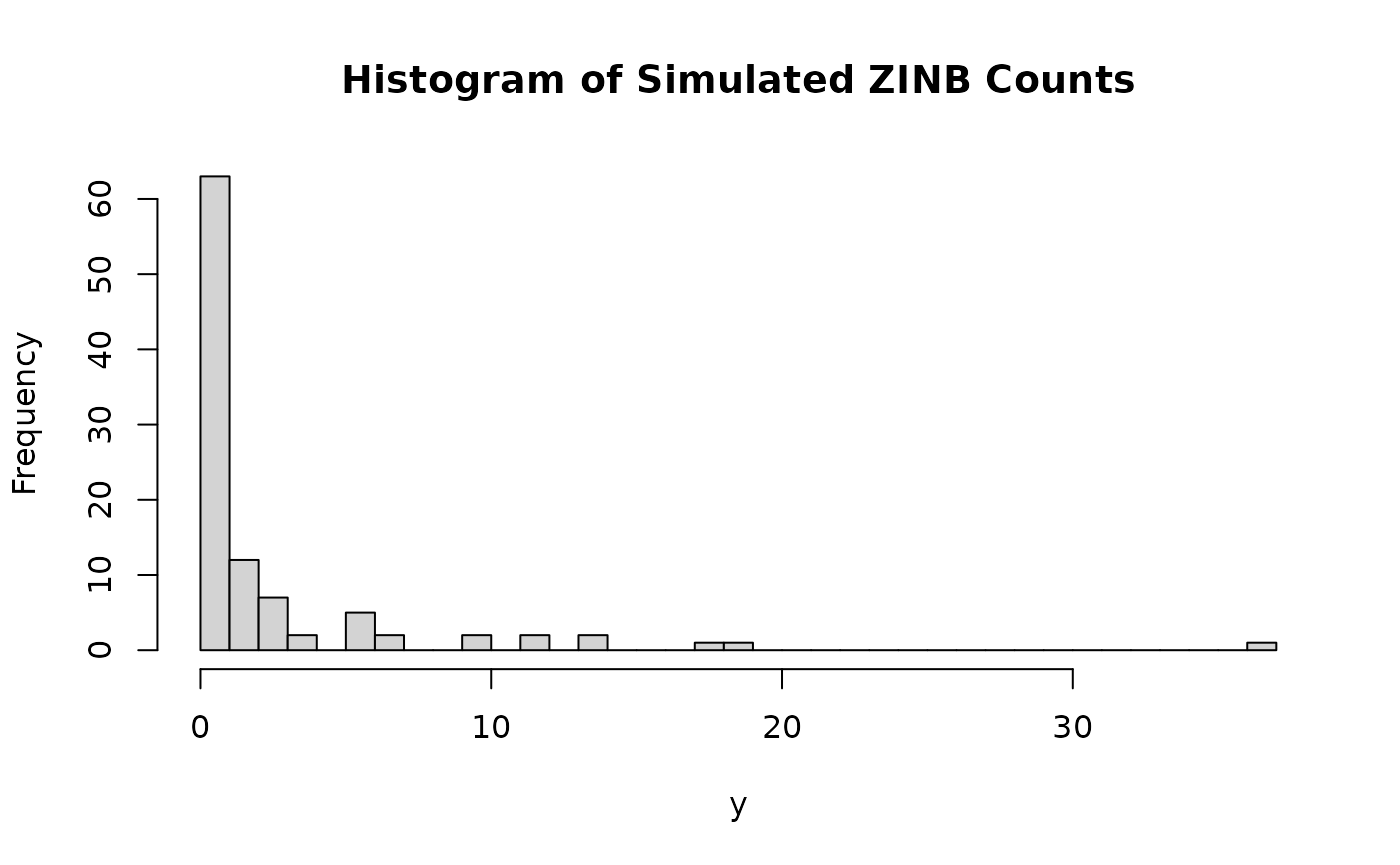

Running ZINB_GP

Now, apply the ZINB_GP function to the simulated data.

# Expanded coordinates for all observations (100 x 2)
# (coords_st was already computed as the expanded grid)

# Now call the function with observation-level covariance matrices:
output <- ZINB_GP(
  X = X,               # 100 x 2
  y = y,               # length 100
  coords = coords,  # 100 x 2 expanded coordinates
  Vs = Vs,         # 100 x 100 covariance matrix
  Vt = Vt,         # 100 x 100 covariance matrix
  Ds = Ds,         # 100 x 100 distance matrix
  Dt = Dt,         # 100 x 100 distance matrix
  M = M,
  nsim = nsim,
  burn = burn,
  save_ypred = TRUE
)

Exploring the Output

Examine the structure of the output and summarize key results.

# Structure of the output
str(output)
#> List of 25
#>  $ Alpha      : num [1:200, 1:2] 1.217 0.251 0.757 1.297 0.625 ...
#>  $ Beta       : num [1:200, 1:2] 0.673 0.804 0.758 0.749 1.038 ...
#>  $ A          : num [1:200, 1:10] 0.0184 0.0731 0.3064 0.4266 -0.2708 ...
#>  $ B          : num [1:200, 1:10] -0.10955 0.08354 0.10053 -0.00428 -0.06613 ...
#>  $ C          : num [1:200, 1:10] 0.511 -0.138 0.143 -0.13 -0.117 ...
#>  $ D          : num [1:200, 1:10] 0.04819 0.02085 -0.03618 0.07592 0.00171 ...
#>  $ Eps1s      : num [1:200, 1:10] -0.00917 -0.07254 0.0228 -0.0171 0.0383 ...
#>  $ Eps2s      : num [1:200, 1:10] 0.0351 -0.2091 0.2494 -0.4704 -0.0108 ...
#>  $ Eps1t      : num [1:200, 1:10] 0.01195 0.00185 0.13576 0.15973 0.08774 ...
#>  $ Eps2t      : num [1:200, 1:10] -0.02788 -0.04098 -0.01125 -0.03955 -0.00724 ...
#>  $ L1t        : num [1:200] 1e-06 1e-06 1e-06 1e-06 1e-06 ...
#>  $ Sigma1t    : num [1:200] 0.144 0.136 0.154 0.131 0.144 ...
#>  $ L2t        : num [1:200] 0.000001 0.000001 0.000001 0.000001 0.103707 ...
#>  $ Sigma2t    : num [1:200] 0.248 0.114 0.115 0.135 0.177 ...
#>  $ Phi_bin    : num [1:200] 4.46 4.46 4.46 4.46 6.23 ...
#>  $ Sigma1s    : num [1:200] 0.295 0.286 0.364 0.393 0.282 ...
#>  $ Phi_nb     : num [1:200] 10.13 8.57 5.83 5.83 5.83 ...
#>  $ Sigma2s    : num [1:200] 0.308 0.257 0.289 0.289 0.232 ...
#>  $ Sigma_eps1s: num [1:200] 0.0454 0.0481 0.052 0.046 0.0483 ...
#>  $ Sigma_eps2s: num [1:200] 0.0734 0.1446 0.169 0.1261 0.1243 ...
#>  $ Sigma_eps1t: num [1:200] 0.0513 0.072 0.0682 0.07 0.056 ...
#>  $ Sigma_eps2t: num [1:200] 0.0447 0.0391 0.0517 0.0421 0.0394 ...
#>  $ R          : num [1:200] 1.38 1.38 1.38 1.37 1.38 ...
#>  $ Y_pred     : num [1:200, 1:100] 0 0 4 4 2 0 3 5 0 0 ...
#>  $ at_risk    : num [1:200, 1:100] 0 0 0 0 1 1 0 0 0 0 ...

# Summary of posterior means (example, adjust based on actual output structure)
if (!is.null(output$Beta)) {
  cat("Posterior means of beta:\n")
  print(colMeans(output$Beta))
}
#> Posterior means of beta:
#> [1] 0.7147136 0.8322667

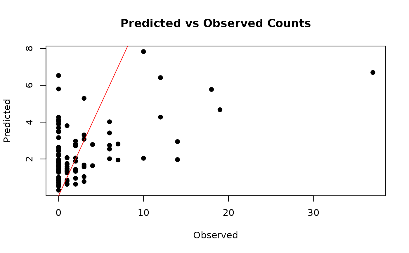
# Plot predicted vs observed values (if available)
if (!is.null(output$Y_pred)) {
  plot(y, colMeans(output$Y_pred), pch = 19, 
       xlab = "Observed", ylab = "Predicted", 
       main = "Predicted vs Observed Counts")
  abline(0, 1, col = "red")
}

Conclusion

This demonstration showcased how to simulate spatial-temporal data and fit a ZINB model with NNGP using the ZINB_GP function. The simulated data included spatial and temporal effects, and the model accounted for zero-inflation and overdispersion. Users can extend this example by adjusting parameters, adding more covariates, or applying it to real data.

Hsin-Hsiung Huang and Mahlon Scott

March 07, 2025